Steps of the GFam pipeline

The GFam pipeline consists of multiple steps. In this section, we will describe what input files does the GFam pipeline operate on, how the steps are executed in order one by one and what output files are produced in the end. First, a short overview of the whole process will be given, followed by a more detailed description of each step.

Overview of a GFam analysis

GFam infers annotations for sequences by first finding a consensus domain architecture for each step, then collecting Gene Ontology terms for each domain in a given domain architecture, and selecting a few more specific ones. Optionally, a Gene Ontology overrepresentation analysis can also be performed on the terms to determine whether some GO terms occur more frequently in a given domain architecture than expected by random chance. Out of these three steps, the calculation of the consensus domain architecture is the most complicated one, as GFam has to account for not only the known domain assignments from InterPro, but also for the possible existence of novel, previously uncharacterised domains. The whole pipeline can be broken to 8+1 steps as follows:

1. Extracting valid gene IDs from the sequence file.
2. Determining a preliminary domain architecture for each sequence by considering known domains from the domain assignment file only.
3. Finding the unassigned regions of each sequence; i.e. the regions that are not assigned to any domain in the preliminary domain architecture.
4. Running an all-against-all BLAST comparison of the unassigned sequence fragments and filtering BLAST results to determine which fragments may correspond to the same novel domain. Such filtering is based primarily on E-values and alignment lengths. At this point, we obtain a graph on the sequence fragments where two fragments are connected if they passed the BLAST filter.
5. Calculating the Jaccard similarity of the sequence fragments based on the connection patterns and removing those connections which have a low Jaccard similarity.
6. Finding the connected components of the remaining graph. Each connected component will correspond to a tentative novel domain.
7. Calculating the consensus domain architecture by merging the preliminary domain architecture with the newly detected novel domains.
8. Selecting a functional label for each of the domain architectures based on a mapping between InterPro domains and Gene Ontology terms.
9. Conducting a Gene Ontology overrepresentation analysis on each of the sequences and their domain architectures to derive the final annotations.

These steps will be described more in detail in the next few subsections.

Step 1 – Extracting valid gene IDs

In this step, the input sequence file is read once and the gene IDs are extracted from the FASTA deflines. The gene ID is assumed to be the first word of the defline. If the deflines in the original FASTA file follow some other format, one can supply a regular expression in the configuration file that can be used to extract the actual ID from the first word of the defline.

Step 2 – Preliminary domain architecture

This step processes the domain assignment file and tries to determine a preliminary domain architecture for each sequence. A preliminary domain architecture considers known domains from InterPro only. Domain architectures for each sequence are determined in isolation, so the domain architecture of one sequence has no effect on another.

For each sequence, we first collect the set of domain assignments from the domain assignment file. Each assignment has a data source (e.g., HMMPfam, Superfamily, HMMSmart and so on), a domain ID according to the schema of the source, the starting and ending indices of the domain in the amino acid chain, an optional InterPro ID to which the domain ID is mapped, and an optional E-value. First, the list is filtered based on E-values, where one might apply different E-value thresholds for different data sources. This leads to a list of trusted domain assignments that are not likely to be artifacts. After that, GFam performs multiple passes on the list of trusted domain assignments, starting with a subset focused on more reliable data sources. Less reliable data sources join in the later stages, and it is possible that some data sources are not considered at all.

During the first pass, one single data source that is giving the highest coverage of the sequence is selected from the most reliable data sources. This data source will be referred to as the primary data source, and the domains of the primary data source will be called the primary assignment. After the first pass, the primary assignment will be extended by domains from other data sources in a greedy manner using the following rules:

1. Larger domains from other data sources will be considered first. (In other words, the remaining assignments not included already in the primary assignment are sorted by length in descending order).
2. Domains are considered one by one for addition to the primary assignment.
3. If a domain is the exact duplicate of some other domain already added (in the sense that it starts and ends at the same amino acid index), the domain is excluded from further consideration.
4. If a domain to be added overlaps with an already added domain from another data source, the domain is excluded from further consideration.
5. If a domain to be added is inserted completely into another domain from the same data source, it is added to the primary assignment and the process continues with the next domain from step 2. Note that the opposite cannot happen as we consider domains in decreasing order of their sizes.
6. If a domain to be added overlaps partially with an already added domain from the same data source, the size of the overlap decides what to do. Overlaps smaller than a given threshold are allowed, the domain will be added and the process continues from step 2. Otherwise, the domain is excluded from further consideration and the process continues from step 2 until there are no more domains left in the current stage.

We call this five-step procedure the expansion of a primary assignment. Remember, GFam works in multiple stages; the first stage creates the primary assignment with a limited set of trusted data sources, the second stage expands the primary assignment with an extended set of data sources, and there might be a third or fourth stage and so on with even more extended sets of data sources. For Arabidopsis thaliana and Arabidopsis lyrata, we found the following strategy to be successful:

1. Assignments from HAMAP, PatternScan, FPrintScan, Seg and Coil are thrown away completely for the following reasons:

   • HAMAP may not be a suitable resource for eukaryotic family annotation as it is geared towards completely sequenced microbial proteome sets and provides manually curated microbial protein families in UniProtKB/Swiss-Prot [4]. For Arabidopsis thaliana, there were only 133 domains annotated by HAMAP and all domains had E-values larger than 0.001.
   • PatternScan and FPrintScan [5] are resources for identifying motifs in a sequence and are not very helpful in understanding larger evolutionary units or domains. The match size ranges between 3 and 103 amino acids for PatternScan and between 4 and 30 amino acids for FPrintScan.
   • Seg and Coil were ignored as these define regions of low compositional complexity and coiled coils, respectively, and are not particularly informative in the context of defining gene families.

2. An E-value threshold of 10^-3 is applied to the remaining data sources, except for Superfamily, HMMPanther, Gene3D and HMMPIR which are taken into account without any thresholding.

   The threshold of 10^-3 was chosen based on the following observation. There are 3,816 domain assignments from HMMPfam with a E-value larger than 0.1, 1,625 assignments with an E-value between 0.1 and 0.01 and 1,650 assignments with an E-value between 0.01 and 0.001. We looked at the type of domains that had an E-value between 0.1 and 0.01 and 0.01 and 0.001. We noticed that at least 80% of the domains are some kind of repeat domains (PPR, Kelch, LLR, TPR etc) or short protein motifs (different types of zinc fingers, EF-hand, HLH etc). It is reasonable to believe that at an E-value less than 0.001, the majority of the domains are likely to be spurious matches due to the sequence nature (low-complex and short) of these domains. We decided to consider domains from HMMPfam that had an E-value of 0.001 or smaller. We may miss but only a handful of real domains if we choose 0.001 as our E-value threshold. However, we would like to point out that the threshold is not hard-wired into GFam, rather it is a parameter than can be tuned for each assignment source to suit the users’ needs.

3. GFam performs three passes on the list of domain assignments obtained up to now. The first and second passes do not consider HMMPanther and Gene3D assignments as they tend to split the sequence too much. The third stage considers all the data sources.

4. The maximum overlap allowed between two domains of the same source (excluding complete insertions which are always accepted) is 30 amino acids. This was based on the distribution of domain overlap lengths for the different resources.

The stages and the E-value thresholds are configurable in the configuration file.

[4]

Lima T, Auchincloss AH, Coudert E, Keller G, Michoud K, Rivoire C, Bulliard V, de Castro E, Lachaize C, Baratin D, Phan I, Bougueleret L and Bairoch A. HAMAP: a database of completely sequenced microbial proteome sets and manually curated microbial protein families in UniProtKB/Swiss-Prot. Nucl Acids Res 37(Database):D471-D478, 2009.

[5]	Scordis P, Flower DR and Attwood TK. FingerPRINTScan: intelligent searching of the PRINTS motif database. Bioinformatics 15(10):799-806, 1999.

Step 3 – Finding unassigned sequence fragments

This step begins the exploration for novel, previously uncharacterised domains among the sequence fragments left uncovered by the preliminary assignment that we calculated in step 2. We improvised on the method described by Haas et al [6] to identify novel domains. The step iterates over each sequence and extract the fragments that are not covered by any of the domains in the preliminary domain assignment. Sequences or fragments that are too short are thrown away, the remaining fragments are written in FASTA format into an intermediary file. The sequence and fragment length thresholds are configurable. For the analysis of A.thaliana and A.lyrata sequences, the minimum fragment length is set to 75 amino acids.

[6]	Haas BJ, Wortman JR, Ronning CM, Hannick LI, Smith RK Jr, Maiti R, Chan AP, Yu C, Farzad M, Wu D, White O, Town CD. Complete reannotation of the Arabidopsis genome: methods, tools, protocols and the final release. BMC Biol 3:7, 2005.

Step 4 – All-against-all BLAST comparison and filtering

This step uses the external NCBI BLAST executables (namely formatdb and blastall) to determine pairwise similarity scores between the unassigned sequence fragments. First, a database is created from all sequence fragments using formatdb in a temporary folder, then a BLAST query is run on the database with the same set of unassigned fragments using blastall -p blastp. Matches with a sequence percent identity or an alignment length less than a given threshold are thrown away, so are matches with an E-value larger than a given threshold. The user may choose between using unnormalised alignment lengths or normalised alignment lengths with various normalisation methods (normalising with the length of the smaller, the larger, the query or the hit sequence).

For A.thaliana and A.lyrata, the following settings were used:

• Minimum sequence identity: 45%
• Minimum normalised alignment length: 0.7 (normalisation done by the length of the query sequence)
• Maximum E-value: 10^-3

Step 5 – Calculation of Jaccard similarity

After the fourth step, we have essentially obtained a graph representation of similarity relations between unassigned sequence fragments. In this graph representation, each sequence fragment is a node, and two fragments are connected by an edge if they passed the BLAST filter in step 4. We will be looking for tightly connected regions in this graph in order to identify sequence fragments that potentially contain the same novel domain. It is a reasonable assumption that if two sequences contain the same novel domain, their neighbour sets in the similarity graph should be very similar. Jaccard similarity is a way of quantifying similarity between nodes in a graph by looking at their neighbour sets. Let i and j denote two nodes in a graph and let denote the set consisting of i itself and i‘s neighbours in the graph. The Jaccard similarity of i and j is then defined as follows:

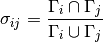
We calculate the Jaccard similarity of each connected pairs of nodes and keep those which have a Jaccard similarity larger than 0.66. This corresponds to keeping pairs where roughly 2/3 of their neighbours are shared. The Jaccard similarity threshold can be adjusted in the configuration file.

Step 6 – Identification of novel domains

Having obtained the graph filtered by Jaccard similarity in step 5, we detect the connected regions of this graph by performing a simple connected component analysis. In other words, sequence fragments corresponding to the same connected component of the filtered graph are assumed to belong to the same novel domain. Note that these novel domains should be treated with care, as some may belong to those that were already characterised in the original input domain assignment file but were filtered in step 2.

Novel domains are given temporary IDs consisting of the string NOVEL and a five-digit numerical identifier; for instance, NOVEL00042 is the 42nd novel domain found during this process. Components containing less than four sequence fragments are not considered novel domains. The size threshold of connected components can be adjusted in the configuration file.

Step 7 – Consensus domain architecture

This step determines the final consensus domain architecture for each sequence by starting out from the preliminary domain architecture obtained in step 2 and extending it with the novel domains found for the given sequence. The consensus domain architectures are written into two files, one containing a simpler flat-file representation of the consensus architectures suitable for further processing, while the other containing a detailed domain architecture description with InterPro IDs and human-readable descriptions for each domain in each sequence. This latter file also lists the primary data source for the sequence, the coverage of the sequence with and without novel domains, and also the number of the stage in which each domain was selected into the consensus assignment.

Step 8 – Functional label assignment

This step tries to assign a functional label to every sequence by looking at the list of its domains and collecting the corresponding Gene Ontology terms using a mapping file that assigns Gene Ontology terms to InterPro IDs. Such a file can be obtained from the InterPro2GO project. For each sequence, the collected Gene Ontology terms are filtered such that only those terms are kept which are either leaf terms (i.e. they have no descendants in the GO tree) or none of their descendants are included in the set of collected terms. These terms are then written in decreasing order of specificity to an output file, where specificity is assessed by the number of domains a given term is assigned to in the InterPro2GO mapping file; terms assigned to a smaller number of domains are considered more specific.

Step 9 – Overrepresentation analysis

This optional step conducts a Gene Ontology overrepresentation analysis on the domain architecture of the sequences given in the input file. For each sequence, we find the Gene Ontology terms corresponding to each of the domains in the consensus domain architecture of the sequence, and check each term using a hypergeometric test to determine whether it is overrepresented within the annotations of the sequence domains or not.

During the overrepresentation analysis, multiple hypergeometric tests are performed to determine the significantly overrepresented terms for a single sequence. GFam lets the user account for the effects of multiple hypothesis testing by correcting the p-values either by controlling the family-wise error rate (FWER) using the Bonferroni or Sidák methods, or by controlling the false discovery rate (FDR) using the Benjamini-Hochberg method.

The result of the overrepresentation analysis is saved into a human-readable text file that lists the overrepresented Gene Ontology terms in increasing order of p-values for each sequence.